Lab 9: Mapping

Initial Hardware and Software Challenges

At the end of last lab, I encountered a cascade of system failures, this lingered into this lab. First, after redownloading my IMU library to fix a dependency issue, the DMP (Digital Motion Processor) was disabled, leaving me unable to use the DMP, which I was unware of. Concurrently, an accidental reassignment of the ToF sensor's XSHUT pin in my configuration file prevented the sensors from booting entirely. Because troubleshooting these hardware and software bugs consumed a significant portion of my lab time, I collaborated with Ananya Jajodia and utilized her robot to complete a portion of the data collection for this lab.

Orientation Control Implementation

To begin mapping, I utilized the orientational PID controller utilizing the IMU's DMP implemented in lab 6. By calculating the error between the target angle and current yaw, the robot could snap to specific orientations.

After observing a decent orientation control, I decide to decrease the P term and increase D term just to get a slower and more reliable turn.

Orientation control proved highly effective for reliable on-axis turns. By commanding the robot through a series of $90^\circ$ turns and driving straight, I tested its odometry by mapping a 2x3 feet rectangular path under the lab table. The results below show a clean, stable path with minimal rotational drift, validating that the positional PID was well-tuned.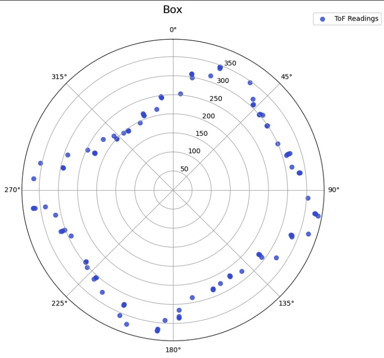

If I was to execute an on-axis turn in the middle of an empty 4x4 meter room, an angular drift of just $3^\circ$ would translate to a positional error of approximately $2\text{m} \times \tan(3^\circ) \approx 0.1\text{m}$ (10 cm) at the walls. Assuming the drift averages out symmetrically across a full $360^\circ$ sweep, the average mapping error would remain extremely low, while the maximum worst-case error at the corners would peak around 10-15 cm.

Angular Speed Control (Alternative)

While positional control worked well, I also wrote a continuous angular speed controller to compare mapping methodologies. This logic utilized a low-pass filter on the Gyro's Z-axis to maintain a constant rotational velocity (e.g., $45^\circ/s$). Due to time constraints recovering from the initial hardware bugs, I did not fully tune this on the physical robot, but the architecture is shown below.

void runSpeedPID(float target_speed) {
    float current_speed = get_gyro_z_lpf(); 
    float e = target_speed - current_speed;
    
    error_total = constrain(error_total + e, -500, 500);
    
    float p_term = Kp_spd * e;
    float i_term = Ki_spd * error_total;
    int motor_out = (int)(p_term + i_term);
    
    if (motor_out > 0) {
        motor_out = constrain(motor_out, 120, 255);
        setMotors(motor_out, -motor_out);
    } else {
        motor_out = constrain(motor_out, -255, -120);
        setMotors(-motor_out, motor_out);
    }
}

Distance Data Collection

To construct the map, I wrote two distinct methods for distance data collection to see which yielded better results.

Method 1: The Quick Scan ($360^\circ$)

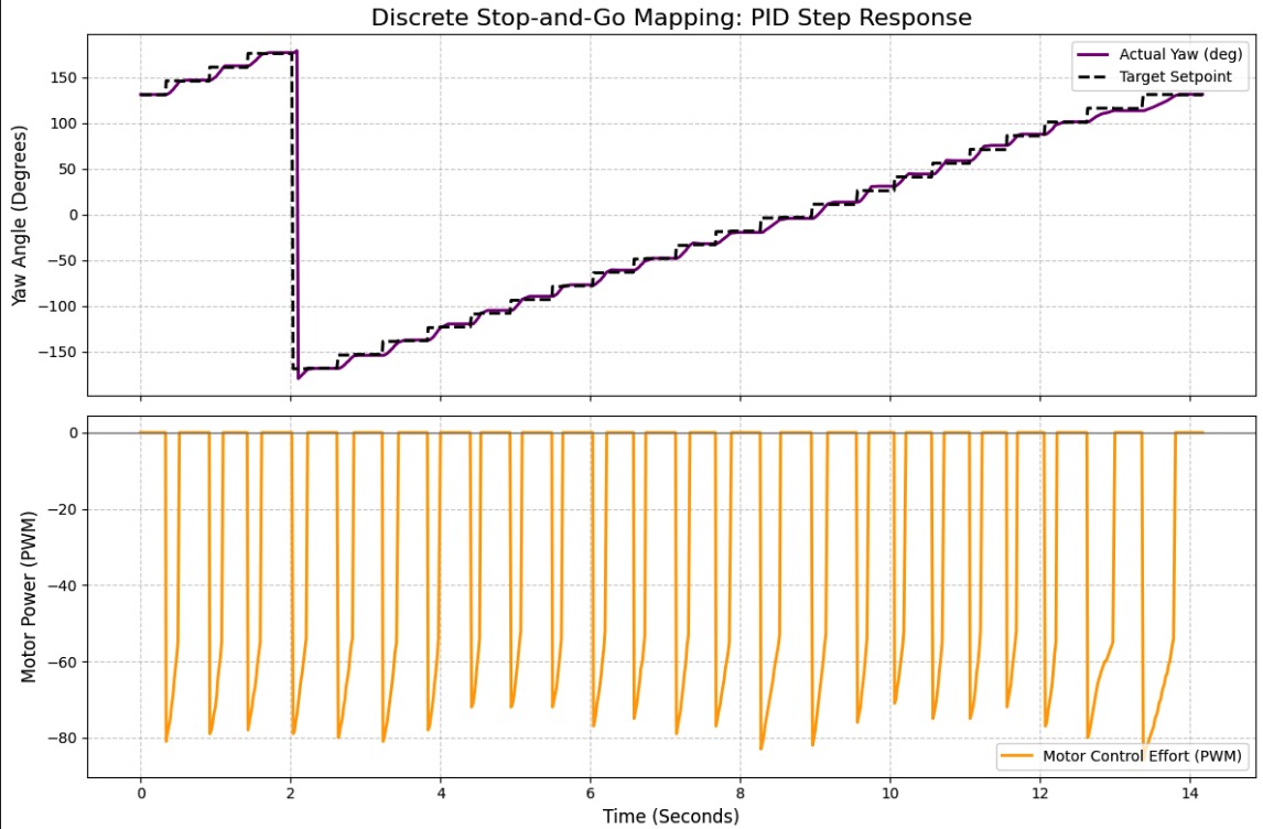
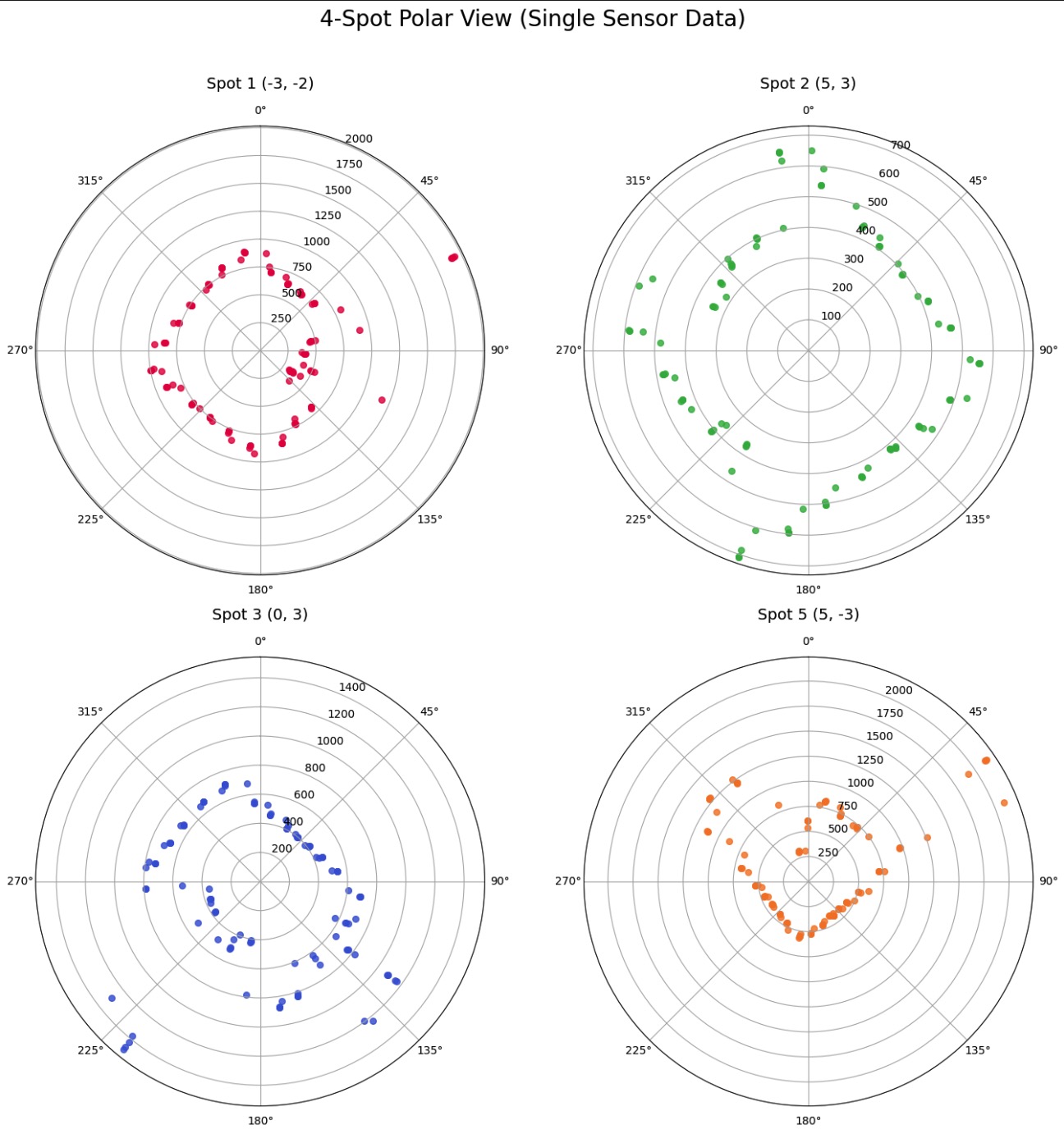
The first approach was a fast, single-rotation scan using a single ToF sensor. The robot used the orientation PID to step in $12^\circ$ increments, rotating a total of $360^\circ$ (30 steps). To prioritize speed, I implemented a tight $\pm 3^\circ$ error tolerance.

Once the robot entered this window, it did not explicitly kill the motors. Because the chassis was still actively vibrating, I needed a way to filter out transient sensor noise. To solve this, I programmed the robot to rapidly record 5 consecutive distance readings at each setpoint and calculate their average. This averaged distance was recorded before the robot moved to the next setpoint, significantly smoothing out the data.

while (rot_counter <= 30 && BLE.central().connected()) {
    readIMUFIFO();
    get_roll_pitch_yaw(0); 
    float curr_yaw = yaw_readings[0];

    float e = curr_yaw - target_turn;
    if (e > 180.0) e -= 360.0;
    else if (e < -180.0) e += 360.0;

    if (abs(e) > 3.0) {
        int motor_out = runPID(e); 
        setMotors(motor_out, -motor_out);
    } else {
        long sum_tof = 0;
        for (int i = 0; i < 5; i++) {
            while (!distanceSensor1.checkForDataReady()) {
            }
            sum_tof += distanceSensor1.getDistance();
            distanceSensor1.clearInterrupt(); 
        }
        tof_data[rot_counter] = sum_tof / 5.0;
        yaw_data[rot_counter] = curr_yaw;
        target_turn += 12.0;
        if (target_turn > 180.0) target_turn -= 360.0; 
        rot_counter++;
    }
}
stopMotors();

While fast, and taking 5-point distance and yaw averaging, this method still occasionally captured noisy data due to the continuous motion.

Data Merging and Final Mapping

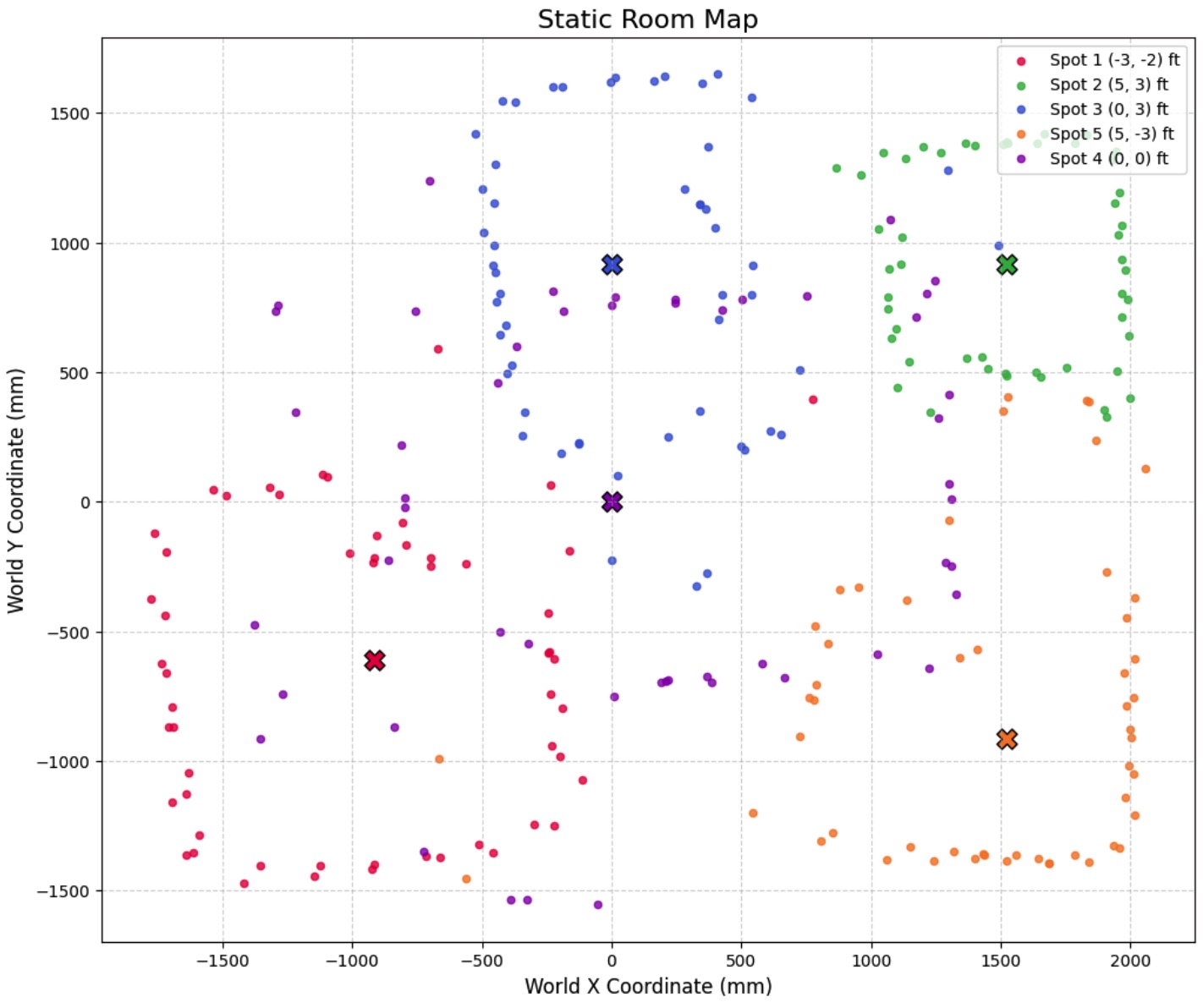
To map the arena using Method 1, I converted the 1D averaged distances into 2D global coordinates. This required two transformation matrices. First, I accounted for the physical offset of the Front ToF sensor relative to the center of rotation.

$$T_{sensor} = \begin{bmatrix} TOF & 0 & 1 \end{bmatrix}$$

Next, a rotational transformation matrix was applied to convert the robot's local angular yaw coordinate into global x^ and y^​ map coordinates based on where the robot was placed in the room.

$$T_{rotation}(\theta) = \begin{bmatrix} \cos\theta & -\sin\theta & robot_x \\ \sin\theta & \cos\theta & robot_y \\ 0 & 0 & 1 \end{bmatrix}$$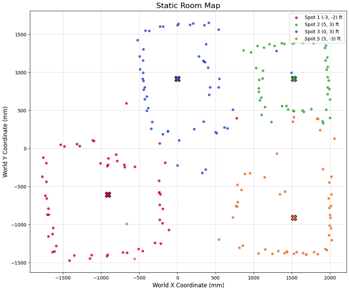

Hardware Inversions and Angle Correction

When initially applying these matrices, the resulting map was mathematically mirrored across the y=−x diagonal and rotated incorrectly. This distortion occurred due to two physical hardware quirks:

Z-Axis Inversion: The IMU is mounted with its Z-axis pointing toward the floor. By the right-hand rule, it reads positive values when rotating clockwise. However, standard trigonometry strictly expects counter-clockwise angles to be positive.

Starting Orientation: The robot began its scans facing the +X axis (0∘), but the base transformation matrix assumed it started facing the +Y axis (90∘).

To fix this globally, I inverted the raw yaw data in Python and locked the target starting angle to 0∘. I also inverted the side sensor's physical offset to prevent it from projecting backward into the mirrored coordinate space.

# 1. Global Hardware Fix (Z-axis points down)
df['Yaw_deg'] = -df['Yaw_deg']

# 2. Lock starting angle to +X axis (0 degrees)
initial_yaw = df['Yaw_deg'].iloc[0]
yaw_bias = 0.0 - initial_yaw
df['Biased_Yaw_deg'] = df['Yaw_deg'] + yaw_bias

# 3. Apply inverted offset for Sensor 2
base_tof2_offset = 90.0 

Method 2: The Dual-Sensor 720∘ Sweep

To maximize accuracy over the quick scan, I wrote a more robust data collection method. This method continuously logged PID telemetry at 20Hz while recording discrete map points every two seconds over a full 720∘ rotation. Because the robot is equipped with two ToF sensors (Front and Side offset by −90∘), executing a 720∘ rotation meant every angle was scanned multiple times. I grouped the wrapped angles and took the .median() of the overlapping points to mathematically filter out odometry drift and transient sensor noise.

The code checks the status of both ToF sensors and saves their distances alongside the exact current yaw from the IMU, ensuring the transformation matrices are mathematically precise.

if (current_time - last_cont_time >= 50 && cont_idx < MAX_CONT_SAMPLES) {
    time_cont[cont_idx] = current_time;
    yaw_cont[cont_idx] = curr_yaw;
    motor_cont[cont_idx] = motor_out;
    p_cont[cont_idx] = p_term;
    i_cont[cont_idx] = i_term;
    d_cont[cont_idx] = d_term;
    
    cont_idx++;
    last_cont_time = current_time;
}

if (current_time - last_rot_time >= 2000 && disc_idx < MAX_DISC_SAMPLES) {
    if (distanceSensor1.checkForDataReady()) {
        tof1_disc[disc_idx] = distanceSensor1.getDistance();
        distanceSensor1.clearInterrupt();
    } else { tof1_disc[disc_idx] = -1; }
    if (distanceSensor2.checkForDataReady()) {
        tof2_disc[disc_idx] = distanceSensor2.getDistance();
        distanceSensor2.clearInterrupt();
    } else { tof2_disc[disc_idx] = -1; }
    
    time_disc[disc_idx] = current_time;
    yaw_disc[disc_idx] = curr_yaw; 
    disc_idx++;

    target_turn += 12.0;
    if (target_turn > 180.0) target_turn -= 360.0;
    
    rot_counter++;
    last_rot_time = current_time;
}

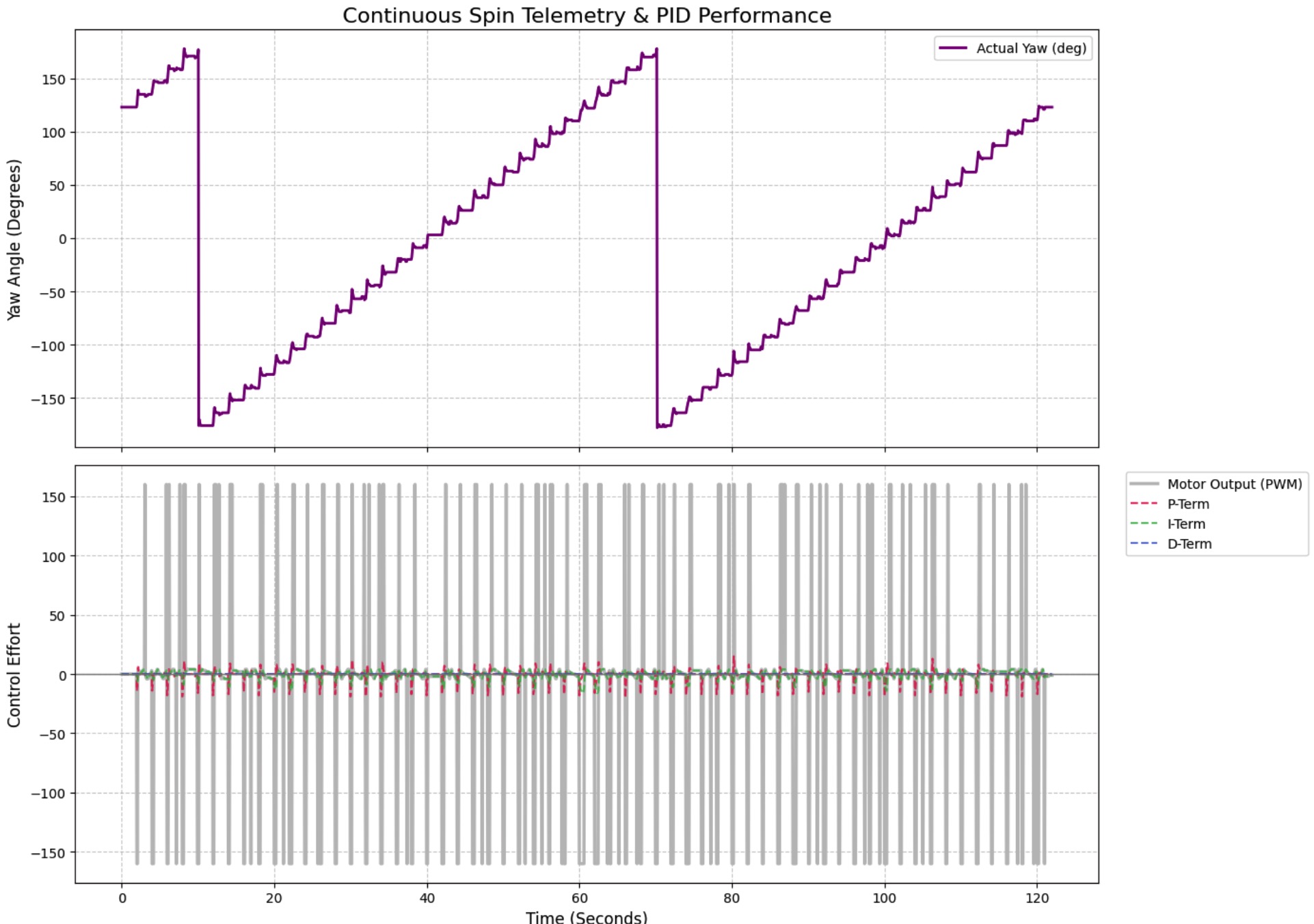
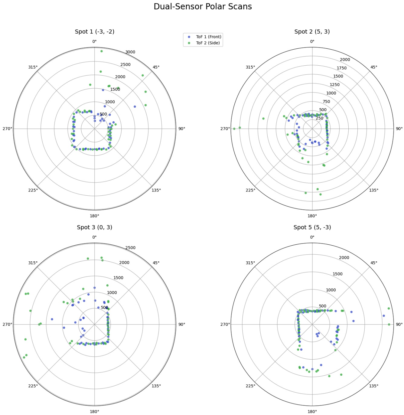
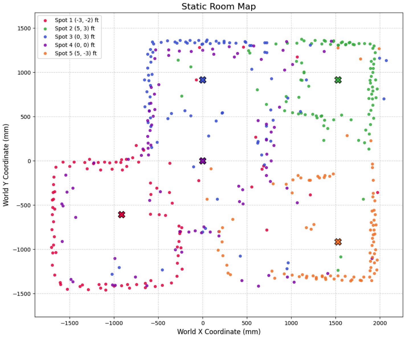
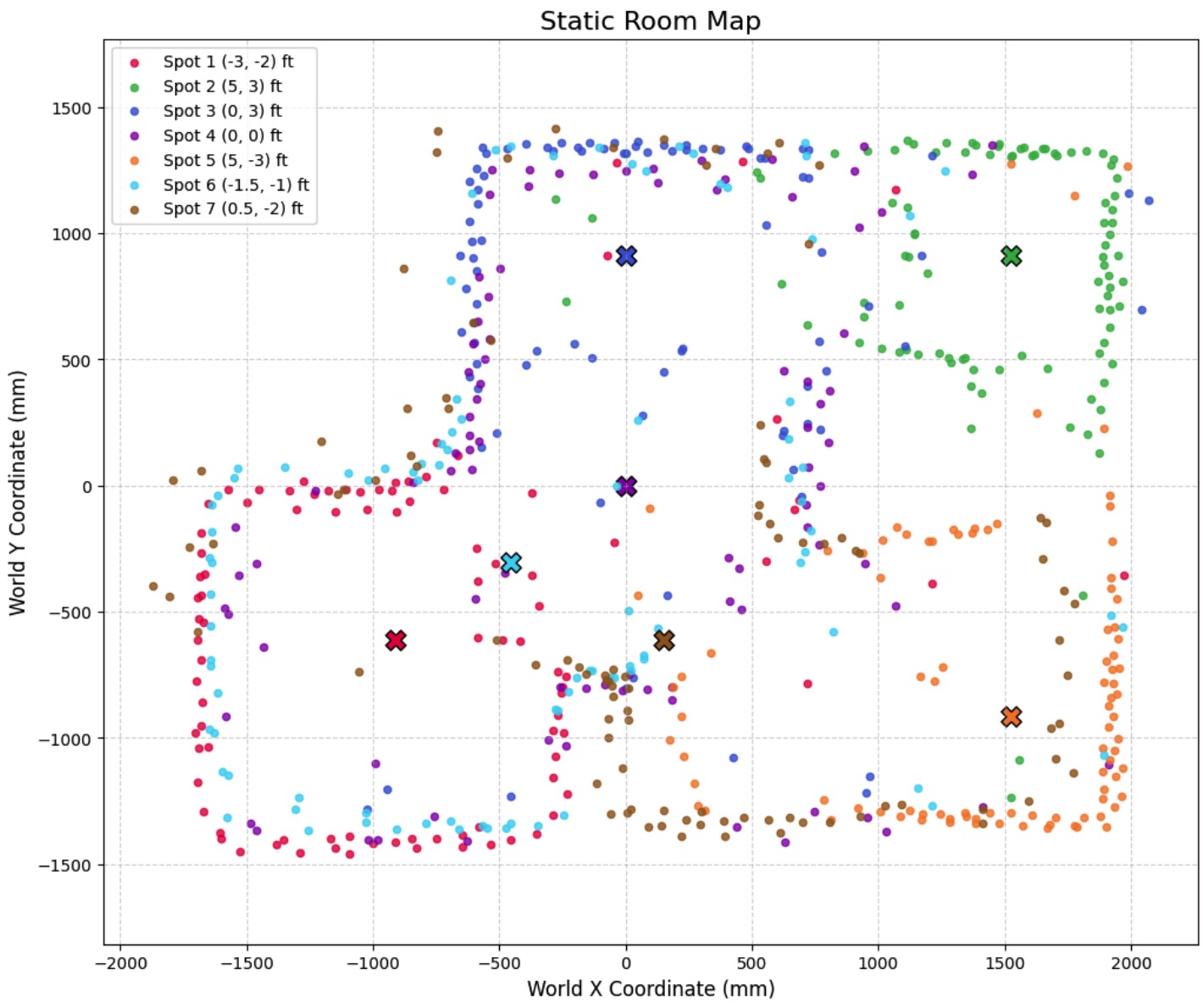
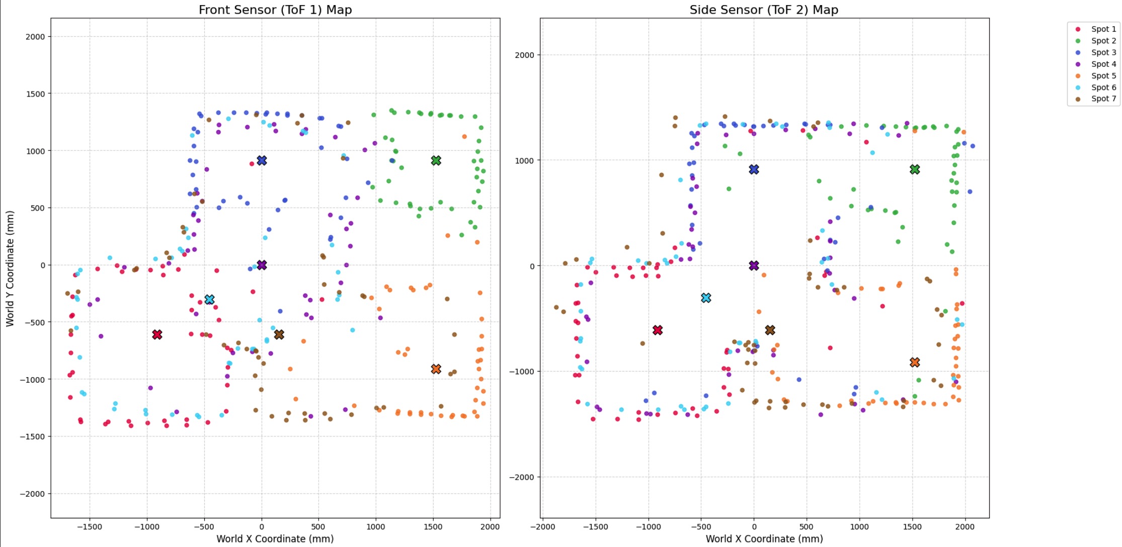
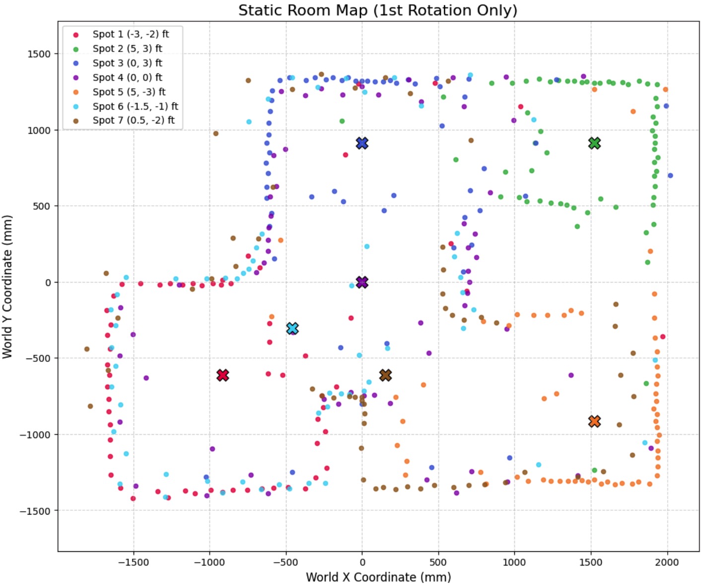
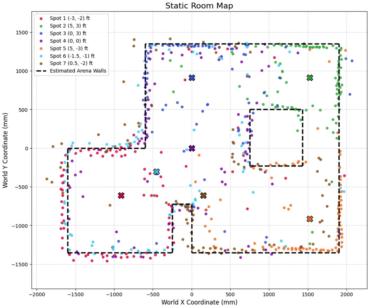
By comparing the generated plots, I was able to optimize the final map. Plotting ToF1 and ToF2 independently revealed that the front sensor was better at detecting the narrow bottom outlet, while the side sensor better captured the top-left square geometry; combining them yielded a more comprehensive view. Interestingly, analyzing the 720∘ dataset showed that isolating just the first 360∘ rotation produced a cleaner map by eliminating the accumulated wheel-slip and odometry drift seen in the second 360 rotation. Implementing these decisions, along with gathering data at two extra spot—(0.5, -2) and (-1.5, -1)—resulted in a final map that accurately reconstructed the arena, aligning with the estimated wall segments.

Collaboration

I collaborated extensively on this project with Ananya Jajodia, and referred to Jack Long and Lucca Correia's site for quality mapping verification. ChatGPT was utilized to assist in formatting Python plotting scripts and organizing graph subplots.